Standford University - CS231n(Convolutional Neural Networks for Visual Recognition)
Stanford University CS231n: Deep Learning for Computer Vision
✔ reference
YouTube
cs231n 2강 Image classification pipeline - YouTube
Lecture 1 | Introduction to Convolutional Neural Networks for Visual Recognition - YouTube
Doc
https://yganalyst.github.io/dl/cs231n_1
https://yerimoh.github.io/DL206/
https://biology-statistics-programming.tistory.com/53
https://velog.io/@cha-suyeon/CS231n-Lecture-9-%EA%B0%95%EC%9D%98-%EC%9A%94%EC%95%BD
https://velog.io/@fbdp1202/CS231n-%EC%A0%95%EB%A6%AC-9.-CNN-Architectures-rp6rx3zy
https://yerimoh.github.io/DL206/
https://velog.io/@cha-suyeon/CS231n-4%EA%B0%95-%EC%A0%95%EB%A6%AC-Introduction-to-Neural-Networks
Regularization
학습 기반의 알고리즘에서 모델이 과적합되지 않도록 손실 함수에 특정한 규제 함수를 더하여 손실 함수가 너무 작아지지 않도록 weight에 페널티를 주는 기법
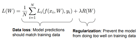
Data loss : 학습용 데이터(training data) 최대한 최적화 → weight가 0이 아니기를 바람 (분류를 해야 하니까)
Regularization : test set 최대한 일반화. → weight가 0이길 바람 → λ : regularization strength, hyperparameter(학습 전에 설정)
λ와 R(W)과 trade-off
training loss와 test set의 generalization loss는 trade off 관계
→ training 결과는 안 좋아지겠지만, 결과적으로 test set의 결과는 좋아진다.
Simple Examples
L2 regularization : $R(W) = \sum\sum{W^2_{k,l}}$
L1 regularization : $R(W) = \sum\sum|{W_{k,l}}|$
Elastic net (L1 + L2) : $R(W) = \sum\sum{\beta W^2_{k,l}} + |W_{k,l}|$
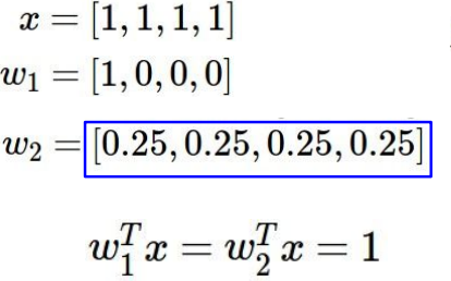
Q. Which of w1 or w2 will the L2 regularizer prefer?
A. 결과는 1로 같지만, L2 regularization은 w2를 더 선호한다. (spread out되어 모든 원소들을 염두하기 때문 → diffuse over everything. 전체적으로 퍼져있다면 복잡하지 않다고 생각)
→ L1 regularization은 w1를 더 선호. (w 중 0이 많을 수록 선호 → 0인 요소가 많을 수록 복잡하지 않다고 생각)
We have some dataset of (x,y)
We have a score function :

We have a loss function:
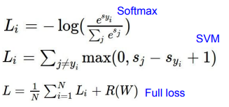
K-NN classifier과 달리 parametric approach의 이점은 parameter를 학습하면 training data를 버릴 수 있다는 점이다.
train data에 대해 잘 예측하는 것이 작은 loss 값을 갖는 것과 동일하다.
Optimization
- parameter W 행렬의 질을 측정
Strategy #1 : Random search → bad idea. 절대 사용 X
Strategy #2 : Follow the slope (gradient) 경사하강법
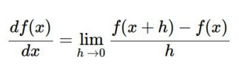
In multiple dimensions, the gradient is the vector of (partial derivatives) along each dimension
The slope in any direction is the dot product of the direction with the gradient
The direction of steepest descent is the negative gradient

f(x+h) → W+h
f(x) → current W
Numeric Gradient 수치 미분
- Slow! Need to loop over all dimensions (W의 모든 원소를 살펴보면서 gradient를 구함)
- Approximate (근사치로 정확한 값이 아니다)
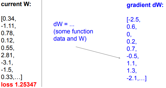
⇒ loss는 그저 W에 대한 function으로 Use calculus to compute an analytic gradient (미분을 통해 구하는 방법)
→ gradient를 나타내는 식을 찾아 dW 계산
In summary:
- Numerical gradient 수치미분: approximate, slow, easy to write :)
- Analytic gradient 해석적 미분: exact :), fast :), error-prone
In practice: Always use analytic gradient, but check implementation with numerical gradient. This is called a gradient check.
→ analytic gradient를 사용하고, 계산이 잘 되었는지 검증을 numerical gradient로 사용.
Stochastic Gradient Descent
전체 데이터셋에서 일부 dataset만 sampling하여 학습에 사용하겠다
Gradient Descent
경사가 하강하는 방향으로 반복해서 gradient를 구함

- Huperparameters
- Weight initialization method:초기값 위치에 따라 수렴 위치&속도가 달라진다.
- Number of steps:steps수가 크면 수행시간이 오래걸리며, 작으면 수렴하기전에 끝날 수 있다.
- Learning rate (step_size):크게 설정하면 optimal 값에 도달하지않고 지나칠 수 있으며, 작으면 시간이 오래 걸린다.
N이 아주 큰 경우 Loss를 계산하는 데 오랜 시간이 걸림
gradient를 계산하려면 N번만큼 더 계산해야함
→ Minibatch로 나눠서 계산하자! : SGD
Mini-batch SGD loop
- sample : a batch of data
- forward : get loss
- backprop : calculate the gradients
- update : parameters using the gradient
W을 임의의 값으로 초기화한 후,
loss와 gradient를 계산하고,
가중치를 gradient의 반대 방향으로 업데이트 (back propagation)
Mini-batch gradient descent
training set 중 일부만을 사용하며, common mini-batch size는 32/64/128/256을 사용한다. (hyperparameter는 아니고, cpu, gpu 수준에 맞게 설정한다, 왜 2의 제곱수를 사용하는가? 벡터 계산시 빠르다)

음의 gradient 방향으로 최적화하는 것이 gradient descent

SGD의 단점
Q. What if loss changes quickly in one direction and slowly in another? What does gradient descent do?
A: Very slow progress along shallow dimension, jitter along steep direction
shallow dimension에서 천천히 이동하며 깊은 방향으로 이동할 때 지그재그형태로 움직인다.
X축 방향은 완만하고, Y축방향은 급격하여서 매우 크게 방향이 튀면서 지그재그 형태로 지점을 찾아가게 됩니다.
Loss function has high condition number: ratio of largest to smallest singular value of the Hessian matrix is large.
Q. What if the loss function has a local minima or saddle point?
A. Zero gradient, gradient descent gets stuck (두 지점 모두 순간적으로 기울기가 0이 되는 지점입니다.)
→ weight 업데이트 할 수 없음
Saddle points much more common in high dimension.

gradients come from minibatches so they can be noisy!
Momentum, AdaGrad, Adam
SGD + Momentum
기존 SGD에서 가속도를 주는 것

continue moving in the general direction as the previous iterations
-Build up “velocity 속도” as a running mean of gradients
-Rho gives “friction 마찰계수”; typically rho=0.9 or 0.99
또한 가속도의 영향을 받으므로 local minima, Saddle points에서도 SGD보다 안전하다
속도가 누적되어 SGD보다 빠르게 이동 가능하다.
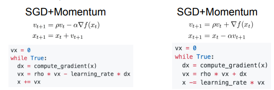
You may see SGD+Momentum formulated different ways, but they are equivalent - give same sequence of x
Nesterov Momentum

momentum update : mu * velocity - learning-rate * gradient Combine gradient at current point with velocity to get step used to update weights
현재 입력값(빨간점)에서 구한 Gradient와 Velocity를 더하여 다음 step를 구한다.
nesterov momentum : momentum step(velocity)를 먼저 계산하고, gradient의 시작점을 정한다
“Look ahead” to the point where updating using velocity would take us; compute gradient there and mix it with velocity to get actual update direction.
Velocity 만큼 움직인 이후에 Gradient를 구하고 이를 더하여 Step를 구한다.


v = 0
for t in range(num_steps) :
dw = compute_gradient(w)
old_v = v
v = rho * v - learning_rate * dw
w -= rho * old_v - (1 + rho) * v
Nesterov는 convex function에서 굉장히 뛰어난 성능을 보임
하지만, Neural Networks 들에 대해서는 별로 성능이 좋지 않음
AdaGrad
각각의 매개변수에 맞게 맞춤형 매개변수 갱신 알고리즘

Added element-wise scaling of the gradient based on the historical sum of squares in each dimension. (누적된 제곱의 합)
“Per-parameter learning rates” or “adaptive learning rates”
Q. What happens with AdaGrad?
A. Progress along “steep” directions is damped (수직축은 gradient가 크므로 업데이트 속도가 낮아진다); progress along “flat” directions is accelerated (수평축은 gradient가 작으므로 업데이트 속도가 빠르다)
Q. What happens to the step size over long time?
A. Decays to zero. learning rate가 0에 가까워지므로 학습이 종료된다.
RMSProp : “Leaky AdaGrad”


과거의 grad_squared를 줄이면서 현재의 gradient를 더 많이 반영하는 방식
(앞에서 온 값을 적용시켜 주어 속도가 줄어드는 문제를 해결)
decay_rate를 곱해준다.
Adam
first_moment는 Momentum
second_moment는 AdaGrad/RMSProp

Sort of like RMSProp with momentum
빨간색은 과거 dw와 현재 dw를 종합하지만 현재의 dw를 더 가중치를 줌으로 Momentum방식을 차용한 형식
파란색은 AdaGrad와 RMSProp방식을 사용하여 dw를 제곱하여 누적함으로 방향정보를 조정한 형식
Q. What happens at first timestep (Assume beta2 = 0.999)?
A: 초기 second_moment 가 0이고 beta2가 1에 가까움. 따라서 한번 업데이트를 한 후에도 second_moment는 여전히 2에 가까워짐. 즉 과거정보인 0값을 많이 참고하여, (분모의 해당하는 값이 0에 가까움에 따라) 초기 gradient step(이동거리)값이 굉장히 커진다.
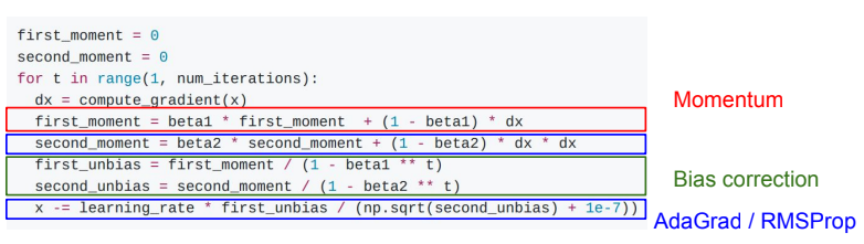
Bias correction for the fact that first and second moment estimates start at zero. (moment값이 0에서 시작하는 문제 개선하고자 bias correction 추가)
Adam with beta1 = 0.9, beta2 = 0.999, and learning_rate = 1e-3 or 5e-4 is a great starting point for many models!
Learning rate schedules
SGD, SGD+Momentum, Adagrad, RMSProp, Adam all have learning rate as a hyperparameter
→ 1st order optimization method라고도 함. (gradient 정보만 사용)
Q. Which one of these learning rates is best to use?
A. In reality, all of these are good learning rates. 어떤 것도 best는 아니다.
Learning Rate Decay
학습률을 점점 감소시켜 가면서 모델의 학습을 안정화시키는 기술

1. Cosine

2. Linear

3. Inverse quare

High initial learning rates can make loss explode; linearly increasing learning rate from 0 over the first ~5,000 iterations can prevent this.
Empirical rule of thumb: If you increase the batch size by N, also scale the initial learning rate by N
높은 초기 학습률은 손실을 폭발적으로 증가시킬 수 있다.
처음부터 5,000회에 걸쳐 0에서 5,000회까지 학습률을 선형적으로 증가시키면 이를 방지 가능하다.
경험적인 규칙 : 배치 크기를 N만큼 늘리면, 초기 학습 속도도 N으로 조정
First-Order Optimization
(1) Use gradient form linear approximation (2) Step to minimize the approximation
Second-Order Optimization
(1) Use gradient and Hessian to form quadratic approximation
(2) Step to the minima of the approximation

장점
conversion 속도 빠름
learning-rate 같은 hyper parameter가 필요하지 않음.
하지만..
Q. Why is this bad for deep learning?
Hessian has O(N^2) elements
Inverting takes O(N^3)
2차 미분 값은 Hessian Matrix 값을 계산해야 함
O(N^2)의 메모리 공간을 필요로 하고 O(N^3)의 Time Complexity를 필요로 함
N = (Tens or Hundreds of) Millions
→ 계산량이 너무 많아 현실적으로 사용 불가
Quasi-Newton methods (BFGS most popular):
instead of inverting the Hessian (O(n^3)),
approximate inverse Hessian with rank 1 updates over time (O(n^2) each).
L-BFGS (limited memory BFGS)
기본적으로 매우 무거운 function
- Does not form/store (메모리 저장 X) the full inverse Hessian
- Usually works very well in full batch, deterministic mode → if you have a single, deterministic f(x) then L-BFGS will probably work very nicely
- Does not transfer very well to mini-batch setting. mini Batch를 사용하지 못해서 실제로 적용하기에 무리가 있음 Gives bad results. Adapting second-order methods to large-scale, stochastic setting is an active area of research.
summary
- Adam is a good default choice in many cases; it often works ok even with constant learning rate
- SGD+Momentum can outperform Adam ,but may require more tuning of LR and schedule
- If you can afford to do full batch updates then try out L-BFGS (and don’t forget to disable all sources of noise)
'🤖 ai logbook' 카테고리의 다른 글
| [NLP/자연어처리] 자연어 처리에서의 순환 신경망 (RNN in Natural Language Processing) (0) | 2023.07.01 |
|---|---|
| [cs231n/Spring 2023] Lecture 4: Neural Networks and Backpropagation (0) | 2023.07.01 |
| [NLP/자연어처리] 정보 검색 & 단어 임베딩(Information Retrieval & Word Embedding) (0) | 2023.07.01 |
| [NLP/자연어처리] 감정 분석 & 문장에 대한 확률 (Sentiment Classification & Probabilities to Sentences) (0) | 2023.06.29 |
| [NLP/자연어처리] 언어 모델에서의 나이브베이즈 (Naive Bayes as a Language Model) (1) | 2023.06.28 |
| [NLP/자연어처리] 언어 모델링(Language Modeling) (0) | 2023.06.28 |
| [NLP/자연어처리] 단어 토큰화(Word Tokenization) (0) | 2023.06.27 |
| [cs231n/Spring 2023] Lecture 2: Image Classification with Linear Classifiers (0) | 2023.06.18 |