
728x90
반응형
Reference
- <파이썬 한권으로 끝내기>, 데싸라면▪빨간색 물고기▪자투리코드, 시대고시기획 시대교육
랜덤포레스트는 배깅과 부스팅보다 더 많은 무작위성을 주어 약한 학습기들을 생성한 후 이를 선형결합하여 최종 학습기를 만드는 방법
수천 개의 변수를 변수 제거 없이 모델링하므로 정확도 측면에서 좋은 성과를 보이는 기법 중 하나
DataSet
https://www.kaggle.com/datasets/yasserh/breast-cancer-dataset
Breast Cancer Dataset
Binary Classification Prediction for type of Breast Cancer
www.kaggle.com
방법
1. scikit-learn의 ensemble.RandomForestClassifier
https://scikit-learn.org/stable/modules/generated/sklearn.ensemble.RandomForestClassifier.html
diagnosis 변수를 이산형 변수로 변환
설명변수 X : area_mean, texture_mean
타깃변수 y : diagnosis
학습데이터 : 평가데이터 = 7 : 3
타깃변수의 클래스 비율 반영되도록 할 것
1. scikit-learn의 ensemble.RandomForestClassifier
class sklearn.ensemble.RandomForestClassifier(n_estimators=100, *, criterion='gini', max_depth=None, min_samples_split=2, min_samples_leaf=1, min_weight_fraction_leaf=0.0, max_features='sqrt', max_leaf_nodes=None, min_impurity_decrease=0.0, bootstrap=True, oob_score=False, n_jobs=None, random_state=None, verbose=0, warm_start=False, class_weight=None, ccp_alpha=0.0, max_samples=None)
더보기
- n_estimators (int): 생성할 트리의 개수입니다. 일반적으로 더 많은 트리를 사용할수록 모델의 성능이 향상될 수 있지만, 계산 비용이 증가하게 됩니다.
- criterion (string, default='gini'): 분류 기준(criterion)으로 'gini' 또는 'entropy'를 선택할 수 있습니다. 'gini'는 지니 불순도를 사용하고, 'entropy'는 엔트로피 불순도를 사용합니다.
- max_depth (int, default=None): 트리의 최대 깊이를 제한합니다. None으로 설정하면 트리의 깊이에 제한이 없습니다.
- min_samples_split (int or float, default=2): 노드를 분할하기 위해 필요한 최소 샘플 수입니다. int로 지정할 경우 해당 개수보다 적은 샘플이 있으면 분할하지 않습니다. float로 지정할 경우 전체 샘플 수에 대한 비율입니다.
- min_samples_leaf (int or float, default=1): 리프 노드가 되기 위해 필요한 최소 샘플 수입니다. min_samples_split과 동일한 의미를 가지지만, 리프 노드에서 적용됩니다.
- max_features (int, float, string or None, default='sqrt'): 각 트리에서 최적의 분할을 위해 고려할 특성의 수를 지정합니다. int로 지정할 경우 해당 수만큼의 특성을 고려합니다. float로 지정할 경우 전체 특성 수에 대한 비율입니다. 'sqrt'는 sqrt(n_features), 'log2'는 log2(n_features), None은 n_features를 의미합니다.
- random_state (int, RandomState instance or None, default=None): 랜덤 시드를 지정하여 재현 가능한 결과를 얻을 수 있습니다. 랜덤한 결정 트리를 생성하는 데 사용됩니다.
import pandas as pd
breast = pd.read_csv('./breast-cancer.csv')

import numpy as np
from sklearn.model_selection import train_test_split

breast["diagnosis"] = np.where(breast["diagnosis"]=="M", 1, 0)
# 이산형 변수로 변환

features = ["area_mean", "texture_mean"]
X = breast[features]
y = breast["diagnosis"]
# 설명변수 X, 타깃변수 y 지정

x_train, x_test, y_train, y_test = train_test_split(X, y, test_size=0.3, stratify=y, random_state=1)
# 학습데이터 : 평가데이터 = 7 : 3
# stratify (array 또는 None, default=None):
# 분할 시 클래스의 분포를 유지하기 위한 배열.
# stratify=y로 지정하면 훈련 세트와 테스트 세트가 원본 데이터와 동일한 클래스 비율을 가지도록 분할된다.
# 일반적으로 분류 문제에서 사용되며, 클래스의 불균형한 분포를 고려하여 훈련 및 테스트 데이터를 나눌 수 있다.

print(x_train.shape, x_test.shape)
print(y_train.shape, y_test.shape)

# (398, 2) (171, 2)
# (398,) (171,)
from sklearn.ensemble import RandomForestClassifier
clf = RandomForestClassifier(n_estimators=100, min_samples_split=5)
# 100개의 결정 트리로 구성된 랜덤 포레스트를 생성
# 노드를 분할하기 위해 최소 5개의 샘플이 필요
pred = clf.fit(x_train, y_train).predict(x_test)
print("정확도 : ", clf.score(x_test, y_test))
# 정확도 : 0.8947368421052632# 부스팅 모델의 예측성능 확인
from sklearn.metrics import confusion_matrix, accuracy_score, precision_score, recall_score, f1_score
pred = clf.predict(x_test)
test_cm = confusion_matrix(y_test, pred)
test_acc = accuracy_score(y_test, pred)
test_prc = precision_score(y_test, pred)
test_rcll = recall_score(y_test, pred)
test_f1 = f1_score(y_test, pred)
print(test_cm)
print('\n')
print('정확도\t{}%'.format(round(test_acc * 100, 2)))
print('정밀도\t{}%'.format(round(test_prc * 100, 2)))
print('재현율\t{}%'.format(round(test_rcll * 100, 2)))
# [[102 5]
# [ 13 51]]
# 정확도 89.47%
# 정밀도 91.07%
# 재현율 79.69%# ROC 커브 시각화하여 AUC 구하기
import matplotlib.pyplot as plt
from sklearn.metrics import RocCurveDisplay, roc_auc_score
RocCurveDisplay.from_estimator(clf, x_test, y_test)
# plot_roc_curve(clf, x_test, y_test)
# plot_roc_curve는 old release of Scikit-learn (version 1.0)에서 제공
# scikit-learn 1.2.2 에서는 RocCurveDisplay 사용
test_auc = roc_auc_score(y_test, pred)
print('auc\t{}%'.format(round(test_auc * 100, 2)))
# auc 87.51%
plt.show()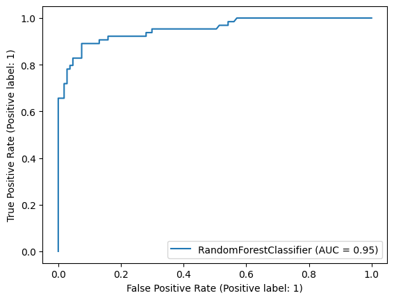
# 사용된 변수들 중 타깃변수에 영향을 가장 많이 준 변수가 무엇인지 확인
# 변수중요도를 통해 확인

importances = clf.feature_importances_

column_nm = pd.DataFrame(["area_mean","texture_mean"]) # 사용한 변수 (X)
feature_importances = pd.concat([column_nm, pd.DataFrame(importances)], axis=1)

feature_importances.columns = ['feature_nm', 'importances']
print(feature_importances)

#      feature_nm  importances
# 0     area_mean      0.72669
# 1  texture_mean      0.27331
# 변수 중요도 시각화
f = features
xtick_label_position = list(range(len(f)))
plt.xticks(xtick_label_position, f)
plt.bar([x for x in range(len(importances))], importances)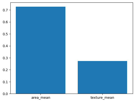
728x90
반응형
'🥇 certification logbook' 카테고리의 다른 글
| [python 데이터 핸들링] 판다스 연습 튜토리얼 - 03_Grouping (0) | 2023.06.13 |
|---|---|
| [python 데이터 핸들링] 판다스 연습 튜토리얼 - 02 Filtering & Sorting (0) | 2023.06.09 |
| [python 데이터 핸들링] 판다스 연습 튜토리얼 - 01 Getting & Knowing Data (0) | 2023.06.08 |
| [ADsP] 비지도학습 - 자기조직화지도(SOM) & 다차원척도법(MDS) (0) | 2023.06.08 |
| 다중 회귀 (Multiple Regression Model) (0) | 2023.06.07 |
| 다항 회귀 (Polynomial Regression Model) (0) | 2023.06.06 |
| 단순 선형 회귀 (Simple Linear Regression Model) (1) | 2023.06.06 |
| 분석환경 설정 (Visual Studio Code + 주피터노트북) (0) | 2023.06.05 |